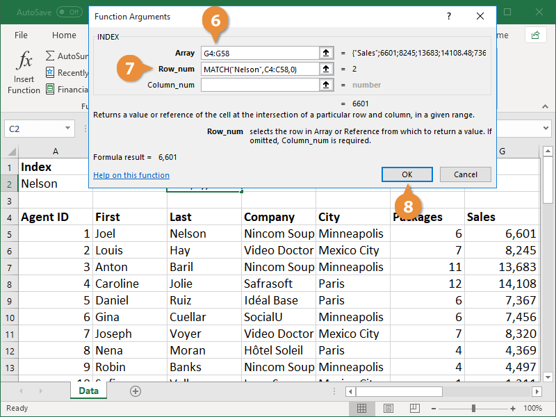
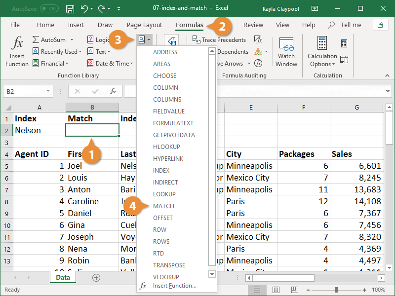
Click the Row_num Box and Nest a Match Function

Click INDEX in the Formula bar. On its own the INDEX function is pretty inflexible because you have to hard key the row and column number and thats why it works better with the MATCH function.

Index And Match In Excel Customguide

Choose or type the Responses range name for the Array argument.

. Select cell for the and cells on the sheet for the. Click the Match_type argument box and type 0. Click the Row_num box and nest a MATCH function.

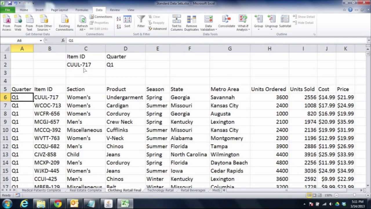
Click the Column_num box and nest a second MATCH function to look up cell D3 on the Mailings sheet in the lookup array A3D3. Select cell B21 for the Lookup_value and cells A3A28 on the Mailings sheet for the Lookup_array. INDEX B2E16MATCH G2A2A160MATCH H2B1E10 You would start out using the Function Arguments dialog box for INDEX.

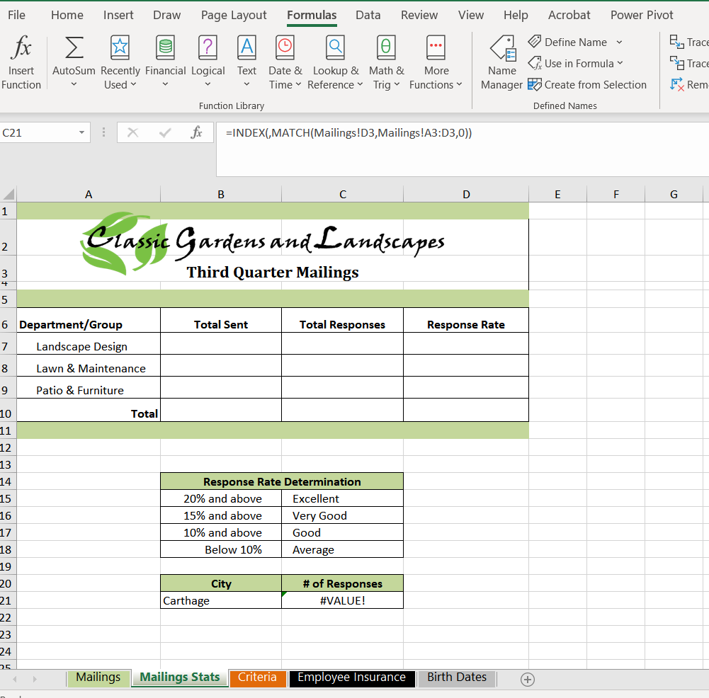
Click the Row_num box and click the Name box arrow. Create a nested INDEX and MATCH function to display the number of responses from a city. You will start with the INDEX function and nest the MATCH function within it.

Select cell B21 for the Lookup_value and cells A3A28 on the Mailings sheet for the Lookup_array. Click the Row_num box and nest a MATCH function. Using the mouse go up to the formula bar and click anywhere inside the word MATCH.

You also calculate insurance statistics and display full names in one cell. For the Array argument type Inventory. Click the Row_num box and nest a MATCH function.

Click the Row_num box and nest a MATCH function. Click the Match_type argument box and type 0. Click the Column_num box and nest a second MATCH function to look up cell D3 on the Mailings sheet in the lookup array A3D3.

The match function I believe then returns the column letter of where that value was found. Click the Row_num box and nest a MATCH function. Click INDEX in the Formula bar.

Choose the Responses range for the Array argument. Click cell C21 start an INDEX function and select the first argument list option. You may have noticed that the INDEX function works in a similar way to the OFFSET function in fact you can often interchange them and achieve the same results.

Click the Row_num box and nest a MATCH function. Click INDEX in the. Click the Mailing Stats sheet tab.

Click cell C21 start an INDEX function and select the first argument list option. Click the Lookup Reference button in the Function Library group. Click INDEX in the Formula bar.

Get Your Custom Essay on excel independent project 6-5 Just from 13Page Order Essay Student. Select the array argument option in the Select Arguments dialog box and click OK. Click the Match_type argument box and type 0 g.

This contains the entry 7. In the Row_num argument box type MATCH. Click the Column_num box and nest a second MATCH function to look up cell D3 on the Mailings sheet in the lookup array A3D3.

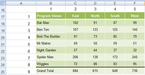
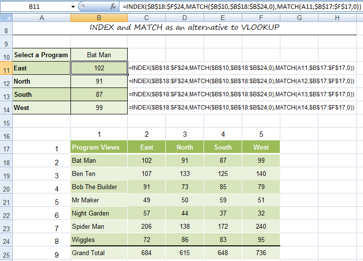
Click the Row_num MATCH B21 Lookup_value A3A28 Mailings Lookup_array Match_type 0. When you copy this nested function into each successive row it increments the A1 to A2 A3 and so on. In this example the formula INDEXA2B742 in cell E2 returns a reference to row 4 of the range A2B7 resulting in cell B5.

Click the Match_type argument box and type 0. Index follows the structure INDEX array row_num col_num area_num. Click the Match_type argument box and type 0.

Click the Lookup Reference button Formulas tab Function Library group and choose INDEX. Click the Match_type argument box and type o. Select cell B21 for the Lookup_value and cells A3A28 on the Mailings sheet for the Lookup_array.

Select the first argument list array row_num column_num and click OK. Box and nest a function. Dont use plagiarized sources.

Click the Row_num box and nest a MATCH function. Choose the Responses range for the Array argument. Select cell B21 for the Lookup_value and cells A3A28 on the Mailings sheet for the Lookup_array.

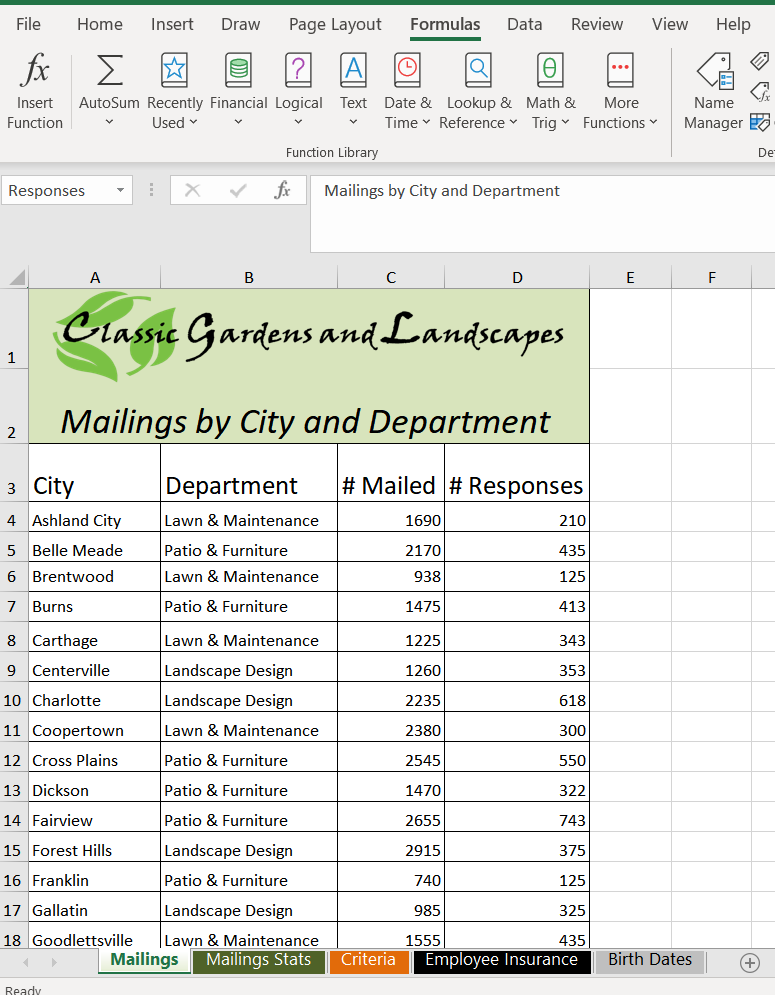
Click the Mailings sheet tab and select and name cells A3D28 as Responses b. Click the Column_num box and nest a second MATCH function to look up cell D3 on the Mailings sheet in the lookup array A303 h. Select cell B21 for the Lookup_value and cells A3A28 on the Mailings sheet for the Lookup_array.

Select cell B21 for the Lookup_value and cells A3A28 on the Mailings sheet for the Lookup_array. Click INDEX in the Formula bar. Select cell B21 for the Lookup_value and cells A3A28 on the Mailings sheet for the Lookup_array.

Click cell B21 and type Carthage. Click the Match_type argument box and type 0. Click the Match_type argument box and type 0.

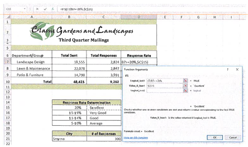
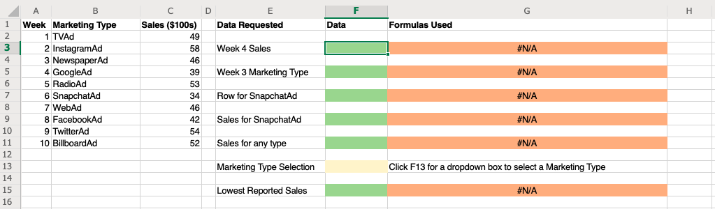
You use SUMIFS and an IFS formula to complete the summary. Select cell B21 for the Lookup_value and cells A3A28 on the Mailings sheet for the Lookup_array. The MATCH function in Excel looks up for a value in a table or array and returns the relative position of the lookup value.

Choose MATCH in the list or choose More Functions to find and select MATCH. Click the Row_num box and nest a MATCH function. Click the Match_type argument box and type 0.

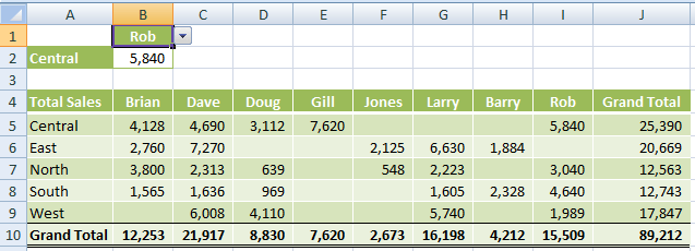
Say that you want to build a formula to do a two-way lookup. Select cell B21 for the Lookup_value and cells A3A28 on the Mailings sheet for the Lookup_array. Click cell C21 start an INDEX function and select the first argument list option.

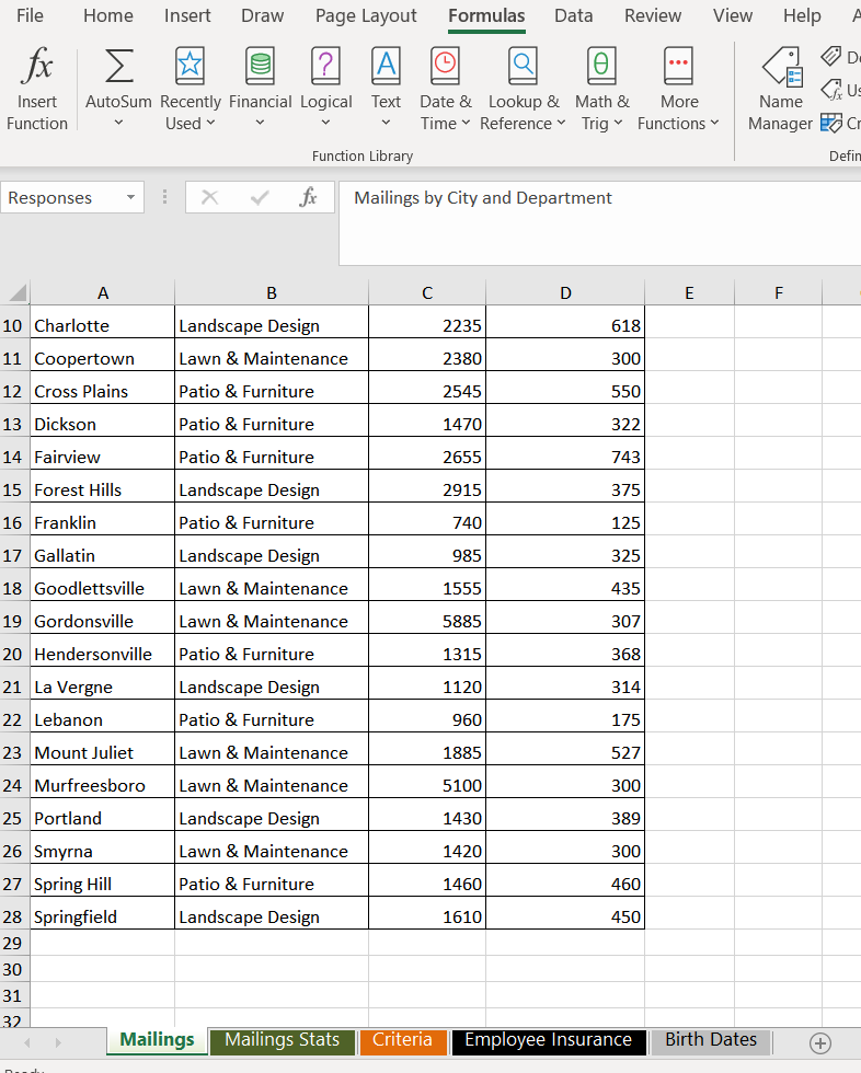
Classic Gardens and Landscapes counts responses to specialty promotions to determine effectiveness. Click cell C21 start an INDEX function and select the first argument list option. Choose the Responses range for the Array argument.

Click cell C21 start an INDEX function and select the first argument list option. Click INDEX in the Formula bar. Click the Row_num box and nest a MATCH function.

Click INDEX in the Formula bar. The index function then displays the value in the column value returned by the match function and in the row specified by the array of cells. Choose the Responses range for the Array argument.

Click the Column_num box and nest a second MATCH function to look up cell D3 on the Mailings sheet in the lookup array A3D3.

Ex2016 Independentproject 6 5 Instructions Using Microsoft Excel 2016 Independent Project 6 5 Independent Project 6 5 Classic Gardens And Landscapes Course Hero

Create A Nested Index And Match Function To Display The Number Of Responses From A City

Solved Please Show Steps On The Index And Match Windows Chegg Com

Create A Nested Index And Match Function To Display The Number Of Responses From A City

Index Match Functions Used Together In Excel

Solved Create A Nested Index And Match Function To Display The Number Of Responses From A City Click The Mailings Sheet Tab And Select And Name Ce Course Hero